Univariate Linear Regression - Boyle's Law

Last Updated: August 29, 2026

In 30 Seconds

ULR-BL is a hands-on machine learning project I built while learning Andrew Ng’s Machine Learning Specialization.

After completing Course 1, Week 1, I wanted to practice what I had learned instead of immediately moving on.

I chose Robert Boyle’s 1662 experimental pressure–volume data and built a univariate linear regression model from scratch in Python.

I implemented the cost function, batch gradient descent, convergence, and prediction, and visualized the cost function in 3D and with a contour plot.

Spark

After learning linear regression, I started looking for a dataset on Kaggle to practice it.

I found many datasets that could work, but I wasn’t satisfied with simply building another prediction model.

For example, I could predict ice cream sales from temperature, but sales depend on many other things too.

I wanted something where the relationship between the two variables actually made sense.

Then I thought of Boyle’s Law.

I had already studied Boyle’s Law and the gas laws in junior college, so I knew that pressure is inversely proportional to volume.

That made it a good dataset for what I wanted to learn.

Vision

I wanted to find out if I could take what I had just learned from Andrew Ng’s course and implement it myself.

I especially wanted to understand the parts I found interesting:

• How the cost function measures error

• How gradient descent updates the weight and bias

• How the model reaches convergence

• What the optimization actually looks like

It was a project for learning by building.

Journey

I found 25 pressure–volume observations from Robert Boyle’s 1662 experiments on the Le Moyne’s College website.

First, I plotted pressure against volume.

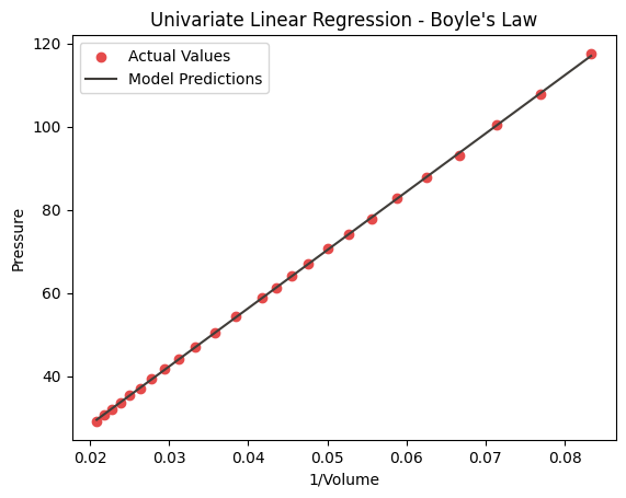
The relationship wasn’t linear, which was expected because Boyle’s Law is:

So I used inverse volume as the input:

and pressure as the target:

I then implemented univariate linear regression from scratch.

The model is:

I started with \(w=0\) and \(b=0\), implemented the cost function and gradients, and used batch gradient descent to learn the parameters.

I used a learning rate of \(\alpha=1\) and a convergence threshold of \(\epsilon=10^{-6}\).

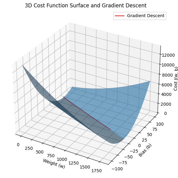
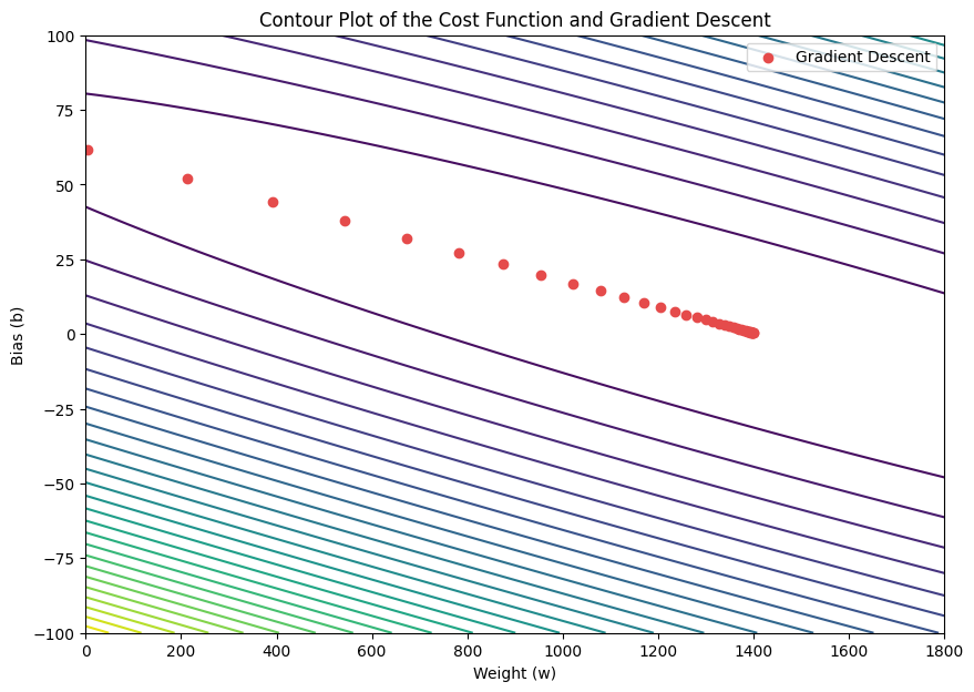
I also plotted the cost function in 3D and created a contour plot to see the gradient descent path.

Visualizations

Challenges

While implementing the cost function, I made a small mistake with the brackets in the denominator. This caused the cost to be much higher than expected.

After checking the implementation, I found the mistake, fixed it, and ran the training again.

It was a simple mistake, but it reminded me that when implementing the mathematics myself, debugging the math is part of the process too.

What I Learned

This project helped me understand univariate linear regression and gradient descent by actually implementing them.

I got a better understanding of how the cost function measures error, how gradient descent updates the parameters, and how convergence determines when to stop the optimization.

The visualizations also helped me connect the equations with what the optimization is actually doing.

Most importantly, I was able to take what I had just learned in the course and build it myself.

Looking Back

This is mainly a learning project.

I wanted to practice the concepts from the course and see if I could implement them on my own.

The Boyle’s Law dataset worked well because I already knew the physical relationship, so I could compare what the model learned with what I expected.

For my next regression project, I want to work with data that has more noise and noticeable residuals.

Links