Predicting Airfoil Self-Noise with Regression
Last Updated:
In 30 Seconds
This is a hands-on machine learning project I built while learning Andrew Ng’s Machine Learning Specialization.
After completing Course 1, Week 2, I wanted to practice what I had learned instead of immediately moving on.
I found NASA’s Airfoil Self-Noise dataset and built a regression project around it.
I implemented Multiple Linear Regression and Polynomial Regression from scratch and trained both using batch gradient descent.
The project gave me a way to take the mathematics from the course and work with it on a real dataset.
Spark
In Week 1, I built a Univariate Linear Regression project using Boyle’s Law.
For Week 2, I wanted something that would let me work with multiple inputs rather than a single input.
While looking for a dataset, I came across NASA’s Airfoil Self-Noise dataset. It contained measurements of airfoil and airflow conditions along with the resulting scaled sound pressure.
That gave me a practical problem to work with.
So I started coding.
Vision
I wanted to use the concepts from Week 2 in one project:
- Multiple inputs
- Feature scaling
- Multiple Linear Regression
- Polynomial features
- Polynomial Regression
- Predictions on unseen data
The goal was simple: take what I had learned and actually make it work.
Journey
I started by inspecting the dataset and understanding its structure.
It contains 1,503 observations, with five input features and one target: scaled sound pressure.
I explored the data and plotted the input features against the target to get a visual sense of the relationships.
I then split the data into training and test sets using an 80/20 split, giving 1,202 training observations and 301 test observations.
Next, I applied Z-score normalization to the input features using statistics calculated from the training data.
After that, I implemented the regression machinery from scratch: prediction, cost calculation, gradient calculation, and batch gradient descent.
Multiple Linear Regression
The first model used all five input features to predict scaled sound pressure.
Compared with my previous Univariate Linear Regression project, the underlying idea was familiar, but now the model had multiple weights and required vector operations.
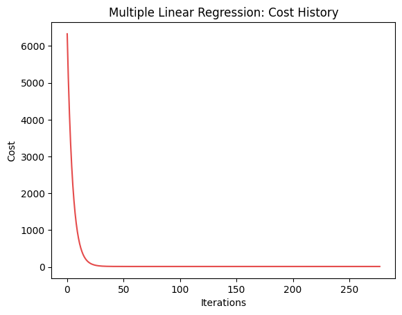
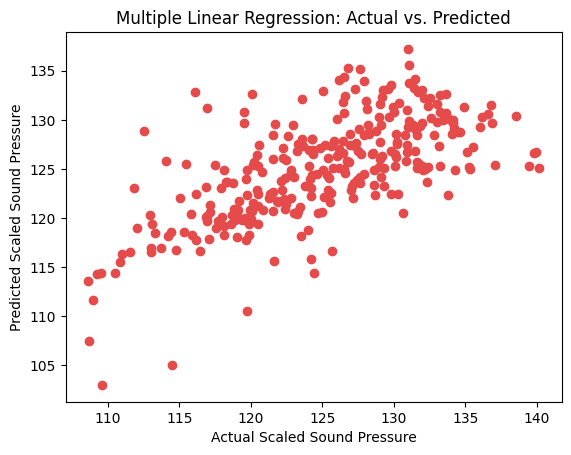
I trained the model using batch gradient descent and evaluated it on the unseen test data.
The test cost was: 12.8558
Polynomial Regression
After training the Multiple Linear Regression model, I wanted to see what happened when the model was given additional polynomial features.
I added the squared version of each of the five original features, giving the model ten features in total.
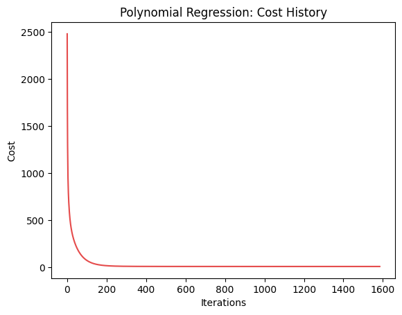
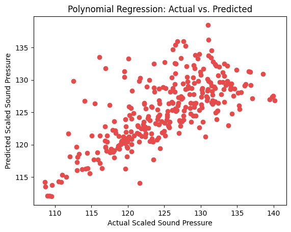
I then trained the model again using the same regression and gradient descent process.
The test cost became: 11.6026
This was 9.75% lower than the Multiple Linear Regression test cost on the same train-test split.
This was useful to see directly because I had learned polynomial features from the mathematics, but now I could see their effect in an actual model.
Visualizations
Challenges
I built the entire project on a phone using Chrome and Kaggle.
The small screen made working with the notebook difficult, and Kaggle occasionally had saving or runtime issues that required me to refresh, restart the kernel, and run the notebook again.
That was the main practical challenge.
What I Learned
Implementing the models gave me a clearer understanding of how the concepts from Week 2 fit together.
Feature scaling became more concrete through implementation. Multiple Linear Regression showed me how the regression model extends from one input to multiple inputs, while polynomial features showed me how transforming inputs can change what the model can represent.
Most importantly, I could now connect the mathematics, code, optimization, and predictions instead of seeing them as separate pieces.
I also moved from one input and one output in Week 1 to five inputs and one output in Week 2.
Looking Back
This project was built to practice the concepts from Andrew Ng’s Machine Learning Specialization, Course 1, Week 2.
I started with the theory and turned it into a working regression project using a real dataset.
It was another step in learning machine learning by actually building with what I learn.